Bivariate Analysis : Difference of Means
Doing T Test in SPSS
The following working examples refer to the
dataset
from the
US General Social Survey 1993
.
1. Analyze ->
Compare Means
-> Independent-Samples T Test
- "independent samples t-test" is usually adopted to compare means
(1 variable, e.g. age or GPA score) between two groups on a categorical
variable in a survey
- if each respondent (i.e. each case) has 2 different scores (i.e.
2 variables) to compare, e.g. GPA of term 1 and GPA of term 2, "
Paired Samples T-Test" should be used
- it is used when 2 measures relate to one another
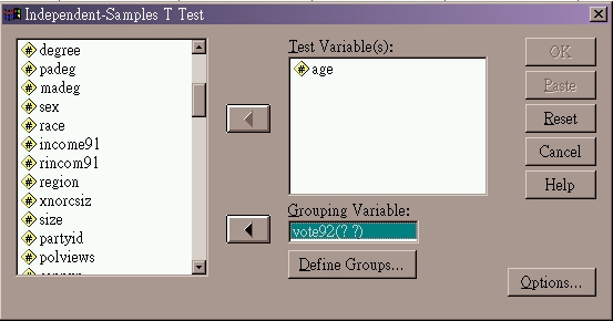
2. Select and put interval (or ratio) scale variable in "
Test Variable(s)" box
3. Select and put categorical variable in "Grouping
Variable" box
- the categorical variable can invovle 2 or more categories
- however, T-Test can only compare 2 groups each time
- define which 2 groups will be included in the comparison by pressing
the Define Groups button
- when there are only 2 categories in the variable, it is still necessary
to define groups

- fill in the codes representing the 2 groups to be compared
- then press Continue
- as in other analyses, press OK
if you want to get the results immediately, or
- press Paste to copy out the command
syntax, then run it in the Syntax window to get the output

4. SPSS Output for T-Test
4.1 We want to know whether mean age of those who voted was differnet from
those who did not vote in the 1992 election
- SPSS will first produce the following table to show the mean age
of the 2 groups in comparison
- in average, those who voted were about 5 years (47.85 - 42.71) older
than those who did not
- from the sample means, we can draw an initial conclusion that voters
were older than non-voters
- however, we are interested more in inferring the sample finding to
the target population, the above conclusion must be tested for statistical
significance
T-Test
Group Statistics
|
VOTE92 Voting in 1992 Election |
N |
Mean |
Std. Deviation |
Std. Error Mean |
|
AGE Age of Respondent |
1 voted |
1028 |
47.85 |
16.953 |
.529 |
|
2 did not vote |
420 |
42.71 |
18.010 |
.879 |
4.2 Test for significance of difference
- the null hypothesis is: voters and non-voters had no difference in
age
- 2 rows contain the same nature of informtion:
t, df,
Sig. (2-tailed) ...
- Equal variances assumed
- Equal variances not assumed
- as you may notice, we have to choose one row of information to believe
, but which one?
- Equal variances assumed or
Equal variances not assumed?
- variances here refer to the variance of each group mean
- rule of decision:
- the null hypothesis is: the variances of the means (2 groups)
are equal
- looking at the pink box, the significance corresponds to the
F-value (in green box)
- if the significance level is greater than 0.05,
the null hypothesis is accepted
- i.e., choose the blue box Equal variances
assumed for information on t-test
- if the significance level is less than or equal to 0.05, the
null hypothesis is rejected
- i.e., choose the yellow box Equal
variances not assumed for information on t-test
- the significance level is 0.202, therefore null hypothesis is accepted
- we have to choose the blue box Equal
variances assumed for information on t-test
- the Sig. (2-tailed) tells us
about the level of significance of the t-value
- the significance shows .000, but it does not mean the probability
is zero, it actually means the significance level is less than 0.0005
- as a convention, we reject the null hypothesis at p
 0.05
0.05
- hence, we may conclude that voters were older than non-voters in
our target population
Independent
Samples Test
|
Levene's Test for Equality of Variances |
t-test for Equality of Means |
|
F |
Sig. |
t |
df |
Sig. (2-tailed) |
Mean Difference |
Std. Error Difference |
95% Confidence Interval of the Difference |
|
Lower |
Upper |
|
AGE Age of Respondent |
Equal variances assumed |
1.631 |
.202 |
5.141 |
1446 |
.000 |
5.14 |
1.000 |
3.179 |
7.102 |
|
Equal variances not assumed |
|
|
5.012 |
737.803 |
.000 |
5.14 |
1.026 |
3.127 |
7.154 |
 0.05
0.05
